On Talking Concretely About Games

Which is to say: without relying on that hollow word, "fun". From a great anti-"gamification" article by Ian Bogost at Gamasutra earlier this year, a passage that I found particularly useful:

... key game mechanics are the operational parts of games that produce an experience of interest, enlightenment, terror, fascination, hope, or any number of other sensations.

(The fun-word-fails-us manifesto, here.)

Book of War Figure Zoom-In

When you see a Book of War figure that looks like this:


Sometimes it helps to keep in mind that it really represents this:


That is: 10 individuals at man-to-man scale, arranged in 2 ranks of 5 files each. Grid spaces in the picture above are 3 feet each (or 3⅓ feet per DMG p. 10, if you prefer). Total length on one side of the formation is 5 spaces × 3 feet/space = 15 feet; i.e., the same as one figure in BOW scale (top picture), ¾ inch base × 20 feet/inch scale = 15 feet.

Early Scaling

As I was forced to dig deep into the Moldvay Basic D&D (1981) rules for the prior blog post, I was surprised to find this at the very end of the book (in Moldvay's 2-page "Dungeon Mastering as a Fine Art" section; literally the last thing in the book before the Credits):

PLAYING SURFACE: Combats are easy to keep track of when large sheets of graph paper, covered with plexiglass or transparent adhesive plastic (contact paper), are used to put the figures on. The best sheets for this use have 1" squares, and the scale of 1" = 5' should be used when moving the figures. [p. B61]

Is this the earliest use in any official D&D rules of the 1" = 5' scale? Both Holmes (earlier; p. 9) and even Mentzer (later; Player's Manual p. 57) still suggest using the 1" = 10 feet scale for miniature play.

I must say (having played by these rules quite a bit back in the day, but not having looked at them in many years) that I'm quite impressed by Moldvay's grasp of the math behind the game. If only he hadn't instituted race-as-class...

On Expected Treasure and XP

Tom Moldvay wrote in his D&D Basic Rulebook (1981):

... most of the experience the characters will get will be from treasure (usually 3/4 or more) [p. B45] *

I think that many old-school players take this as a statement of original design intent regarding the old D&D treasure types and experience system. I'm going to disagree with that, and claim: (a) this statement by Moldvay is descriptive and not normative, and (b) while it's accurate for Moldvay's B/X rules, it does not match other editions of D&D. (Note: All discussion below is in terms of by-the-book D&D gold-standard economy.)


Arneson's OD&D

Let's look at OD&D first. Below you'll see a table of all the hostile monster types (those appearing in dungeons) from Vol-2, p. 3. Each has its standard number appearing, experience point value (per Sup-I, Greyhawk), and expected value from its treasure type (including the requirement that the in-Lair % chance be rolled; as stated on Vol-2, p. 23). Then a ratio for expected value of the treasure versus monster XP is made. (Download full .xls spreadsheet here.)


The end result: Over all of these monster types, there is a GP:XP ratio of 1.5; that is, only about 3:2 in favor of the treasure XP. A clear majority of monsters actually give more XP from the monster than the treasure (about 20 of 30). Note that there are two extraordinary outliers: Dragons (ratio 8:1) and Medusae (ratio 23:1!); if you remove these two outliers from the list, then the overall ratio dips to just 0.8 (i.e., actually less treasure than monster XP). Another way of looking at this, perhaps -- roughly 40% of all the available treasure in the game comes from Dragons, and until the PCs are high enough level to be hunting dragons, their XP will mostly not be coming from treasure. (If played purely according to these random charts.)

Side observation -- The majority of most treasure value comes solely from the Jewelry component. By my calculations, almost all of the OD&D treasure types have between 55% to 85% of their average value coming from Jewelry (average 70%; with outlier Type G, a low 20% of its value from jewelry). Or in other words: If you miss the Jewelry component roll for a treasure type, then you've missed about 2/3 of the nominal value of that treasure type, on average. Or again: Making the Jewelry roll approximately triples the total value from any treasure type.

Other note -- You might look at the XP example of the troll in Vol-1 ("7,000 G.P. + 700 for killing the troll = 7,700" [p. 18]) and say, "hey, that's evidence that OD&D gives about 10% XP for monsters". Except that the example is doubly impossible from the listed monster/treasure tables: (a) trolls number appearing is 2-12 (1 being impossible), and (b) troll treasure type D has at best 1-6 thousand gold pieces (7,000 being impossible). According to my stats, the average result would be to get 7 trolls for 4,550 XP (7×650 per Greyhawk) and a total 3,743 gp value, i.e., as we're saying, expect more XP for the trolls than the treasure. (Also: This example refers to trolls as being "7th level", whereas the monster levels in Vol-3 only go up 6th, so the example is pretty disconnected from the rest of the rules.) Keep in mind that if we used pre-Greyhawk XP (HD×100), then things would be even more skewed in favor of the monster XP.


Moldvay's B/X

Let's try this again for Moldvay's B/X rules. Now, two huge changes will occur at this point. One: The large-scale numbers appearing have been dramatically reduced for the numerous humanoid types (usually dividing by about ten; e.g., men/bandits from 30-300 in OD&D to 3-30 in B/X, etc.). Two: The Lair % statistic has been entirely removed, so presumably any time the larger number of creatures appears, they get their full treasure type valuation. See the results of that below (or spreadsheet for this here):


Now: Over the same core hostile monster types, the GP:XP ratio is close to 3; i.e., a 3:1 relationship of treasure to monster XP -- or in other words, exactly the "usually 3/4" from treasure as Moldvay asserted (see quote at top). Most monster types (about 25 of 30) do indeed give more XP from their treasure than from the monster. While dragons and medusae still have excellent GP:XP ratios, now the far and away outlier is actually Men, with an astounding 108:1 ratio in favor of their treasure! (Analysis: Type A is an excellent type of treasure;the number appearing was divided by 10 from OD&D; and the frequency of treasure was multiplied 6-fold by dropping the low 15% Lair chance.)

Side observation -- Moldvay presents a list of "average values (in gold pieces) of each treasure type" [p. B45], and Moldvay's averages are extremely accurate. (They match very nicely to my numbers in the linked spreadsheet.)

Other notes -- In general, the following are all copied directly from OD&D: (a) Monster treasure types. (b) Treasure type contents (with the addition of new electrum & platinum categories). (c) Monster numbers appearing, for types other than the multitudinous humanoids. (d) The XP values for monsters. (e) Dungeon unguarded treasure tables. However, gem and jewelry values have distinctly dropped by abandoning parts of the generation procedure (gems in a batch "increasing value", and jewelry high-end exceptional rolls).


Treasure in the Dungeon

Now, the preceding was based just on looking at the core "numbers appearing" and "treasure types" from OD&D, which are generally supposed to be just for wilderness encounters. We might ask the obvious question of what's supposed to be the case in the dungeon, but the situation there is enormously more murky. Unfortunately, all of the classic versions of D&D leave this issue almost entirely unspecified and in the realm of pure DM fiat.

• OD&D states multiple times that monster numbers should be scaled to size of the PC party (Vol-2, p. 4; and Vol-3, p. 11). The listed numbers should be "primarily only for out-door encounters" (Vol-2, p. 4); and treasure types are only applicable to "those cases where the encounter takes place in the 'Lair'" (Vol-2, p. 23). In the dungeon, all we are given is that creature numbers are "modified by type" (Vol-3, p. 11; more discussion here). Dungeon treasure might possibly be generated on level-based tables (Vol-3, p. 7), although in later editions of D&D, those tables are generally indicated as for unguarded treasure only. (Note: If used for that purpose, then the average GP:XP is even lower, 0.7 by my calculations, i.e., about the same as the treasure types sans dragons: spreadsheet here.)


• Holmes D&D keeps the same treasure types; he removes all of the numbers appearing in the monster entries (esp., all of the hundreds of humanoids); but he adds specific numbers for the dungeon wandering monster tables (usually on the order of 1d6 or so). But as far as dungeon treasure goes, he gives a short nod to OD&D and then punts to another product entirely:

  The TREASURE TYPES TABLE (shown hereafter) is recommended for use only when there are exceptionally large numbers of low level monsters guarding them, or if the monsters are of exceptional strength (such as dragons). A good guide to the amount of treasure any given monster should be guarding is given in the MONSTER & TREASURE ASSORTMENTS (available from TSR or your retailer). [Holmes D&D, p. 22]



• Moldvay's B/X still maintains the same treasure types; and he merges the numbers appearing into two high/low categories (but again: dividing the truly large numbers by about 10). He says that the higher numbers are for when "met in in the monster's lair (home) or in the wilderness", and regarding treasure types, "in general, treasure is usually found in a monster's lair (home)" [p. B30]. This linkage is reiterated again later:

  Treasures A through O are large, and generally only for use when large numbers or fairly difficult monsters are encountered. The lairs of most human-like monsters contain at least the number of creatures given as the wilderness "No. Appearing" (the number in parentheses). [p. B45]
  



• However, having said that twice so far (that full Treasure Types are for large, lair-wilderness numbers only), Moldvay then contradicts this with his dungeon stocking procedure. Having rolled a small, random dungeon-wandering sized encounter, he says, "If treasure is in a room with a monster, use the Treasure Type for that monster (given in the monster description) to find the treasure in the room.)" [p. B52] Zounds!


• Frank Mentzer's DM's Rulebook basically copies the Moldvay language on treasure types. "When the Treasure Type is a letter from A to O, that should only be the treasure found in a full lair (the Wilderness No. Appearing -- the number in parentheses in the monster description)" [p. 40]. However, his dungeon-stocking procedure apparently switches back to the OD&D rule -- it deletes any mention of monster Treasure Types, and instead references the same short level-based random treasure table: "The amount of treasure can be determined by using the random Treasures Table..." [p. 47] (I guess I would consider this a proper fix to the overly-generous and contradictory Moldvay rule.)

So we see that in most versions of D&D, the preponderance of the evidence is that Treasure Types are actually not to be used for standard dungeon-based small numbers of monsters, but only for large wilderness-equivalent numbers in the "lair". Which is a rather significant misstep, based on our standard dungeon-centric use case. But that data is the best we have for expected XP ratio from treasure/monsters -- and as we've seen for OD&D, if we use the dungeon level-based treasure tables, then the ratio is even lower (more from monsters than treasure). In neither case does it seem like this was an advance design consideration.

(Notice that I haven't worked out AD&D numbers for this discussion: it would be quite a bit harder, since in that work Gygax switched from one-letter-type-per-monster to a mixture of several different combined letters per monster. That said, I'm assuming that the ratios are about the same as in OD&D, since the numbers appearing, in-lair %, etc., are generally copied directly from that work. With the possibly large wild card of awarding XP for usage of magic items.)


Conclusions

Here are some conclusions that I would offer, based on this evidence:

• Arneson probably didn't plan out any statistics like this in advance for the original system. And probably Gygax never actually used random treasure tables at all in his games. (I'd say they're both notorious for not actually using the published rules; and the vagueness of dungeon numbers and treasure speaks to the lack of any specific system for that in the first place.)


• Moldvay, however, shows an exquisite awareness of the average results produced by the treasure table system (as evidenced by his correct 3/4 ratio statement; and listing the correct average values for each treasure type, unique to his rules). That said, this could not have been an advance design decision, because he simply copied all the legacy types and valuations from OD&D (and does an across-the-board deletion of Lair %, and reduces the larger numbers appearing).
  

Let's accept that the D&D treasure and experience amounts were not initially designed with any particular ratio of XP from treasure versus monsters. But let's say that you want that, to promote certain desirable types of gameplay (such as rewarding treasure-acquisition from stealth and trickery, for example). Then you might select from one of the following possible options: (a) Follow Moldvay in deleting in-Lair % checks, and dividing humanoid lair numbers by about 10. (b) Ignore the in-lair dictums for treasure types entirely, and award the whole Treasure Type even for small numbers like 1-6 orcs. (c) Boost the XP value from treasure, perhaps awarding 10 XP per GP, or something like that (also accelerating advancement). (d) Shift all of the XP away from monster-killing, adding the same value to their treasure-acquisition awards (if that's what you want to promote, might as well go whole-hog, eh?)


* Thanks to Tavis and Kipper at the ODD boards for reminding me where this statement came from.

And additional thanks to UWS Guy and DHBoggs for informing me in the comments that the OD&D treasure type system was the work of Dave Arneson.

(Photo by Falashad, under CC2.)

Testing Balanced Dice Power

The point of this not too far-fetched scenario is that chi-square is a test of rather low power; its ability to reject the null hypothesis, even when the null hypothesis is patently false, is quite weak. And the smaller the size of the sample, the weaker it is. -- Richard Lowry, Vassar College

One of the things that's gotten a lot of interest on this blog is my presentation of how to test for fair (balanced) dice -- a statistical application of the well-known Pearson's chi-square test. (See prior posts on the subject here, here, and here.) One of the things I said about the test, early in the first post was this:

It has a significance level of 5%; that is, there's a 5% chance for a die that's actually perfectly balanced to fail this test (Type I error). There's also some chance for a crooked die to accidentally pass the test, but that probability is a sliding function of how crooked the die is (Type II error). A graph could be shown for that possibility, but I've omitted it here (usually referred to as the "power curve" for the test).

And when I said, "a graph could be shown for that possibility, but I've omitted it here", that was, of course, code-speak for "I have no f*ing idea how to compute that or what it would look like". At least one person later expressed interest in seeing it, so at that point my goose was cooked, so to speak. (Thank you very much, Mr. JohnF.)

Therefore, what I did recently was sit down and write a short Java program to simulate the appropriate power-test results by random simulation, and I'll present them below. This investigation was quite instructional to me personally, because it was a significant step outside my comfort zone, and not something that I could find explicitly done anywhere online or in any textbook I could access.

Let me first explain some testing terminology, so that we can be careful with it. In statistical hypothesis testing, there is defined a "null hypothesis" (nothing is changed from normal), and a competing "alternative hypothesis" (something is changed from normal). Usually we, the experimenter, are in some way rooting for the alternative hypothesis (as in: this drug makes sick people recover faster, so now we can build a manufacturing plant and start selling it). To be safe, hypothesis tests are therefore set up with a very high burden of proof for the alternative hypothesis. The end result is technically one of either "reject the null hypothesis" or "do not reject the null hypothesis" -- and without extraordinary evidence to the contrary, we "do not reject the null hypothesis" (i.e., assume nothing has changed by default: compare to other notions like burden of proof and Occam's razor).

Mathematically for us, the null hypothesis will be a specific fixed number (probability distribution), and the alternative hypothesis will be that something varies from that expected number. For dice-testing, therefore, the null hypothesis is actually that the die is perfectly balanced (no face different than the others; e.g., 1/6 chance each for a d6). The alternative hypothesis is that the die is malformed in some way (i.e., at least one face with an altered chance of appearing). So based on what I just said above, if the test says that the die is unbalanced (reject the null hypothesis), then you can pretty much take that to the bank. But if the test fails to say that -- then we've got an open question as to what, exactly, that tells us. (Hence, this investigation.)

Here are three important terms in a hypothesis test: n, α (alpha), and β (beta). The value n is the sample size; how many times we roll the die for our test (previously I'd said the test is justified for a minimum of n=5 times the faces on the die; i.e., 30 rolls for a d6, 100 rolls for a d20). Value α is the chance of a false positive (Type I error; rejecting the null hypothesis when it's true; apparently getting evidence of an unfair die when it's actually balanced; also called the "significance level"). Value β is the chance of a false negative (Type II error; non-rejection of the null hypothesis when it's false; finding no evidence of an unfair die when it's actually unbalanced; also 1 - "power level"). More on these error types here.

Going into the test, you can pick any 2 of the 3 (the last term is logically determined by the others). Obviously, we would like both α and β to be as low as possible, but neither can be zero. A higher sample size n, of course, always helps us. But for a fixed sample size n lowering α increases β and vice-versa (it is, therefore, a balancing act). In practice, you usually set n to whatever size you can best achieve (time and grant-money permitting), and α to the industry-standard of 5%.

In theory you could solve for the resulting β value -- except that to do so would require perfect knowledge of the balance of the die you're testing -- and of course, that's what you're trying to determine in the first place with the hypothesis test.

So: here's what you'll be getting below. Assume that your die has a single odd face that is biased in some way (different probability than the others: I'll call this special probability P0), and that the other faces all have equal probability from what's left. We'll make a graph for every possible value of P0 (on the x-axis), and compare it to the simulated value of 1-β (so that higher is better, on the y-axis), and see what that looks like. This is called the "power curve" for the test; it's an important analysis, but usually glossed over in introductory statistics courses.

(Side note: Is the "one odd face" model realistic? Probably not: if you shave down one edge, then you'll change the likelihood of at least two faces appearing. If one face appears less, then the opposite face should come up more. But at least this model gives us an impression of the test's power.)

This is accomplished by the following Java program (GPL v.2 license). The program takes a certain type of die and fixed levels for n and α, and outputs a bunch of (x,y) values, where x = P0 and y = Power of the test for that odd-face-probability value. These values I copy into a spreadsheet program and then generate a chart from the results. (The program only makes one table at a time; to change die-sides, n, α, or anything else, you've got to manually edit & recompile).

DicePowerCurve.java

Below are the results for a d6, across several increasing values of n (number of rolls we might perform). Or click here for a PDF with some additional charts:

This shape is basically what we expect from a "power curve" chart: something of a "V" shape, with the bottom-point at the value of an actual balanced face (here, 1/6 = 0.17). The y-axis shows the power of the test: the probability of rejecting the null hypothesis in the test (i.e., a finding for the alternative: that the die is unbalanced). It's more likely for this to happen the more skewed the die is (further left or right). It's less likely for this to happen if the die is minimally skewed or actually balanced (near the center). The fact that in each case it actually bottoms out at a value of approximately 0.05 -- that is, the α value: what we initially chose as the chance of a Type I error (rejection when it's balanced) -- gives us confidence that the simulation is giving us accurate results.

So, what is the major lesson here? At moderately low values of n, this test freaking sucks. Look at the chart for n=50 (first one above) and consider, for example, the case where one face never shows up at all (P0=0.00). The test only has an 88% chance of reporting that die as being unbalanced. It's even worse at n=30 (not shown here), which we previously said was a permissible number of rolls for the test; then the power is only about 40%. That is, for n=30, the test only has a 40% chance of telling any difference between a d5 and a d6!

The n=50 d6 power curve has a very gentle bend to it, and what we would like is something with a much sharper dip -- ideally a low chance of rejection at P0=1/6 (17%), a high chance away from it, and as rapid a switchover as possible. For that purpose, n=100 looks a little better, and n=200 even better than that. At n=500 we've really got something: nearly 100% chance of rejection if the special face comes up less than 10% or over 25% of the time. (The PDF shows even sharper power curves for n=1000 and n=2000.)

Let's try that again for a d20 (which would be balanced at a value of P0=0.05):

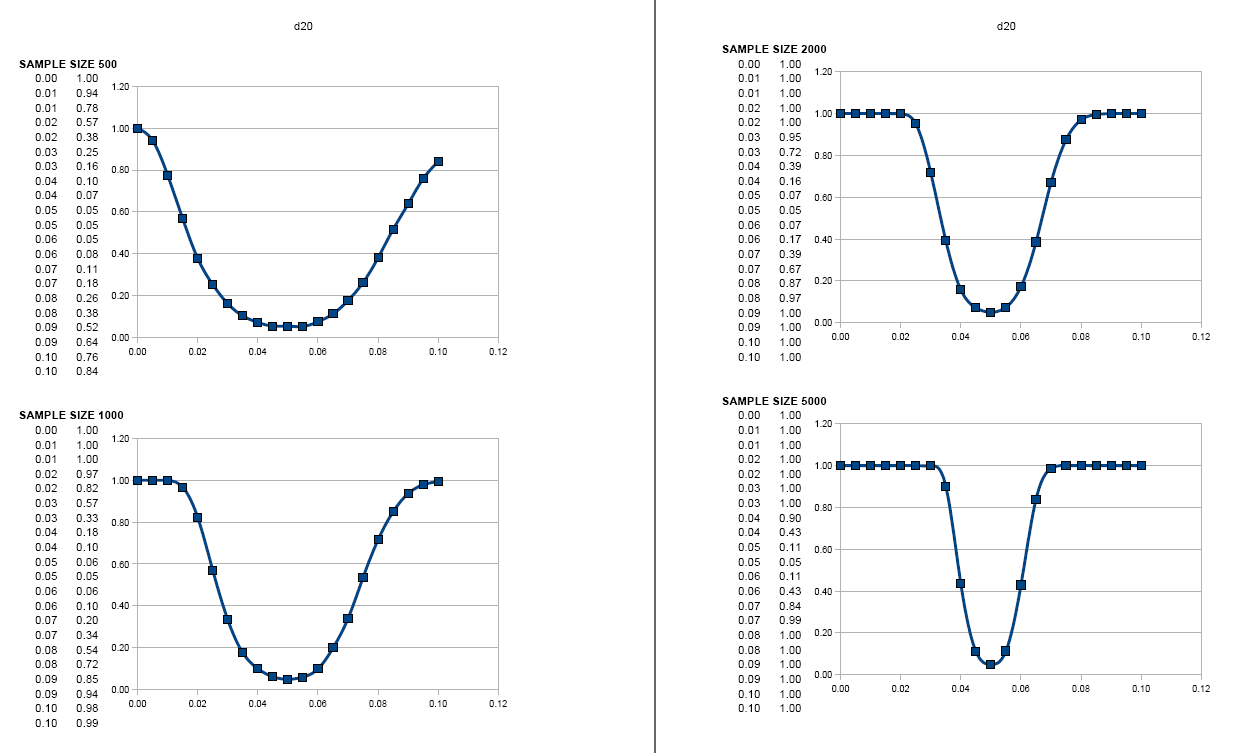Here, I didn't even bother to show anything less than n=500, since the curves below that point are just dreadful (shown in the PDF again linked here). For example, at n=100 (previously the nominal minimum number of rolls), the chance of the test detecting the difference between a d19 and a d20 (i.e. one face missing) is only 16%! So in this case, although we have the same low false positive rate of α=5%, we have a sky-high false negative rate of β=84%. While a finding of "unbalanced" is one that we can count on, a finding of "not unbalanced" tells us almost nothing: it would usually do that anyway, even for a die entirely missing one or more faces.

This is honestly not something that I realized before doing the simulation experiment.

Take-away lesson is this, I think: The bare-minimum number of rolls given previously (5 times faces on the die) is pretty much useless for the test to be powerful enough to actually detect an unbalanced die. For a d6, I wouldn't want to use any less than n=100 as a minimum (and ideally something like n=500 if you're serious about it). For a d20, n=500 would be a useful minimum (and at least several thousand to find reasonably small variations). So realize that it takes a lot of rolling to have a chance of actually detecting unbalanced dice; look at the charts above and decide for yourself how small a bias you want to have a chance of identifying.

---

Postscript: Again, this is an analysis that is frequently overlooked, and if you got through this whole post, then you probably have a deeper understanding of the power of Pearson's chi-square test than even some professional statisticians (I dare say). For example, in the old Dragon magazine article on the subject (Dragon #78, Oct-1983), writer D.G. Weeks completely screwed up on this point. He wrote:

If your chi-square is less than the value in column one (labelled .10), the die is almost certainly fair (or close enough for any reasonable purpose).

Well, that's just totally false. At minimal sample sizes, the test is of such low power, that the die can be almost certainly unfair and still pass the criteria. Furthermore, Weeks presented the possibility of a test for a given suspected die-face frequency and included it in the attached BASIC computer program, in doing so vastly confusing the issue of what's the null and what's the alternative hypothesis. To wit:

In this case it might make more sense to test directly whether this observation is really accurate, rather than simply making the general test described earlier. If what you suspect is true, a specialized test will show the bias more readily...

What I would say is that this would actually prove the bias LESS readily, since your suspicion has now become the null hypothesis, and non-rejection of the null hypothesis tells us next to nothing about the die -- because that's what happens by default anyway, and the test is so very low-powered. In fact, Weeks is making precisely the mistake that we are being warned about by Professor Lowry in the quote at the very top of this blog post (read more at that link if you like: "it is a terrible idea to accept the null hypothesis upon failing to find a significant result in a one-dimensional chi-square test..."). Don't you make the same error!

Book of War Core Rules Justification Part 2

I usually don't trust myself to do a computation just once. Customarily I try to construct: (1) a procedural computer simulation, and (2) a formal math calculation, and if the two results synch up together, then I can have some confidence in them.

So last time I presented the Java computer-simulation version of the Book of War Core Rules mechanic (the 3/4/5/6 target on d6 to score a hit on a 1:10 scale figure wearing no armor/leather/chain/plate). For me, that's always the more concrete demonstration, but the truth is that we don't really need it: we can also do a direct math calculation.

Let's just do one case as an example. Say you've got normal men attacking normal men in chain mail (no shield: AC 5). Per the OD&D hit chart, those men hit on a score of 14 or more on d20; i.e. (excluding the lower 13), 7 chances in 20, or probability 7/20 = 0.35. From prior work, we know that on average it takes 1.52 successful hits to kill a 1-HD man. (See the two proofs of that here and here). The one attack roll per BOW turn represents 3 D&D rounds, with 5 men along the front line attacking, but it takes 10 kills before a whole mass figure is eliminated. So the expected value (probability) of figure kills each turn is:

0.35 × 1/1.52 × 3 × 5 / 10 = 0.345

Note that all the factors after the initial probability basically cancel out; so, the probability of a hit in D&D is basically the same as the probability for a figure-hit at our chosen BOW scale! So nice. In any event, we can convert this probability to a d6 target value using our standard formula:

7-6*p = 7-6*(0.345) = 4.93 ≈ 5

And of course, that's the same "AH 5" value that we've been claiming all along for targets in chain mail armor. Moreover, we can do this for every possible AC value if we want to be really careful with it. Here's the result:

(Click above for a PDF version. Or click here for an Excel spreadsheet, if you want to tweak or check the calculations.) Okay, so it turns out that the totally correct conversion isn't exactly just a divide-by-3 operation, but it's really close. Leather & shield should technically be AH5 according to this, like basic chain mail. And we can also see what should happen for mega-hardened AC values at the bottom of the chart (clearly unhittable by normal men in OD&D).

This table actually appears in the Book of War Optional Rules section at the back, in case anyone wants to be totally precise with that. But for most purposes, I'm very happy with the 3/4/5/6 per armor-type Core Rule, being exceedingly simple and elegant. The other thing noted in the table is that while in OD&D, normal men can hit AC -1 on a perfect 20, this 1-in-20 chance is negligible in terms of d6 success rates; so, for example, I'm pretty happy with the language in the heroic-level section wherein I summarize this as, "characters with negative ACs are given AH 7" (or greater) [BOW, p. 13].


One final thing to keep in mind: We've now twice-confirmed that the expected values of BOW combat are the same as D&D combat played tens or hundreds of men at a time (i.e., on average, BOW combat produces the same results as D&D combat). But what could not be kept identical with the scale-switching was the variance of the results; that is, BOW combat should be more "swingy" than if you really played out mass combat at the D&D man-to-man scale. (My estimate is that standard deviation has been multiplied by a factor of √15 = 3.87 , since one BOW roll represents 15 D&D attacks; but maybe less than that because damage hit point rolls have been abstracted out of the equation?) Personally I don't mind that, since it says that we're giving the underdog a bit more chance to come out on top, say.

Nevertheless, in practice we've actually found that games at equal point-values (and no enormous mistakes by either player) tend to be almost supernaturally even; we've seen lots of games that come down to the last two opposing figures on the table, with a single hit determining the victor (even if the game swung back-and-forth before that, over the course of play). So our confidence that Book of War is a game balanced unto itself is also quite high. More on why that's the case a bit later.

Book of War Core Rules Justification Part 1

So last week, I presented the Book of War Core Rules in an Open Game Content format, and discussed why the scales were determined as they were. I pointed out that we use a fundamental conversion rate of 1 BOW turn = 3 D&D rounds, and the basic combat mechanic is to roll a d6 for mass attacks (with success on 3/4/5/6 for no armor/leather/chain/plate, i.e., divide d20 target numbers by 3 and round down). So now you could ask two questions:

Why the 1 turn = 3 rounds equivalence? Am I just slavishly copying what Gygax set down in Swords & Spells (and Niles in Battlesystem)? Answer: No, I was ready to use something else if it created an elegant and statistically correct mechanic. But, it turns out that the 1:3 rate is particularly special.

And, granted that the 3/4/5/6 hit rule (divide targets by 3) is convenient and easy to remember, but is it an accurate portrayal of mass scale attacks (noting that hit points, 1:10 men, and 1:3 rounds have all been abstracted away)? Answer: Yes, as you can see below.

So, take a step back to the point before I'd settled on either the core hit mechanic or the 1:3 round equivalence. I wrote a short computer program that simulates a couple million random D&D-style combats and investigates the results. You can check out the Java code version for the program below (released under GPL v.2):

BOWCoreRule.java

What this program does is create a separate table for each possible round ratio from 1 to 6. Each table is a matrix of different key ACs (in the none/leather/chain/plate categories) and possible target Hit Dice. For each combination we run 10,000 rounds of simulated combat each. (We assume that attackers are all normal men/1st level; hit dice and damage are 6-sided as in OD&D; and that 1:10 figures are meeting along a 5-man front face, such that 5 attacks are delivered each round. When one man dies, another steps up from behind him to take his place.)

We then take the total number of men killed, and turn that into an average number of figures killed per turn (i.e., mean or "expected value"; which is also a probability-per-turn if between 0 and 1). For multi-Hit-Dice types, multiply by the HD to pro-rate this to a chance of a "figure hit" per turn. Finally, convert that probability to a d6 target value, by computing (7-6*p) and rounding off. The output appears in the following text document:

BOWCoreRule.txt

Now, most of those numbers are kind of a garbled mess, except that one table in particular looks quite memorable, namely this one:



Core Mechanic @ 3 round(s) per turn:

HD
AC 1 2 3 4 5 6 7 8
--------------------
10 3 3 2 2 2 2 2 2
7 4 4 4 3 3 3 3 3
4 5 5 5 5 5 4 4 4
1 6 6 6 6 6 6 6 6

So this immediately attracted me, in that if we set the time scale at 1 turn = 3 rounds, then you get this super-easy to memorize core mechanic (reading down the first few columns): a figure of normal men need to roll a 3/4/5/6, on average, to score a "figure hit" against a 1- or 2-HD target, in each of the basic armor categories. And that's really why I chose it.

A few comments: Note that a single die roll here actually represents 15 normal D&D attacks (sword-thrusts or arrow-shots; 5 men in the front line × 3 rounds per turn). When I say a "figure hit", that's actually the elimination of 10 Hit Dice worth of damage (which is a whole 1:10 figure eliminated for 1st-level types, or half of a 2-HD group, etc.)

And the other thing that can be noted here is that technically, it gets marginally easier to score a hit against higher-HD types (by the 8-HD level, most of the target numbers have decremented by one). But we already knew this: Higher Hit Dice are actually devalued in terms of hits taken (from two years ago: proof one; proof two). Short explanation: Low-HD monsters "waste" more received damage as they quickly dip below zero hit points; while high-HD types will suffer full value from the same hits. Nevertheless, in this context I'm happy to gloss over the technicality for the sake of simplicity: we give high-HD types full value in terms of hits taken, thereby giving them an extra bit of a boost.


If you like (and have the programming capacity), then you can take this little simulation and modify it to check out the results if any of your assumptions about basic D&D combat differ from mine. (Or check my code to make sure I didn't make any mistakes.) Here's one modification that immediately springs to mind: What if you play D&D by post-Greyhawk (OD&D Supplement I) rules, wherein hit dice are 8-sided, and weapons like a sword, battleaxe, or polearm also do 8-sided damage? Let's see the modified results of that right now:

Core Mechanic @ 3 round(s) per turn:
[Modified for 8-sided hits and damage]

HD
AC 1 2 3 4 5 6 7 8
--------------------
10 4 3 2 2 2 2 2 2
7 4 4 4 3 3 3 3 3
4 5 5 5 5 5 5 4 4
1 6 6 6 6 6 6 6 6

Well, as you might guess, that's basically the exact same thing with one notable exception: 1-HD men in "no armor" would be hit on a 4 instead of a 3. (And I guess there's one other number that's different if you look closely enough, at the 6HD level.) So as long as your battles don't commonly feature lots of completely unarmored normal men joining the fight, then you can call this "close enough", and be confident that the Book of War system functions exactly the same, on average, as any other version of classic D&D.