The point of this not too far-fetched scenario is that chi-square is a test of rather low power; its ability to reject the null hypothesis, even when the null hypothesis is patently false, is quite weak. And the smaller the size of the sample, the weaker it is. -- Richard Lowry, Vassar College
It has a significance level of 5%; that is, there's a 5% chance for a die that's actually perfectly balanced to fail this test (Type I error). There's also some chance for a crooked die to accidentally pass the test, but that probability is a sliding function of how crooked the die is (Type II error). A graph could be shown for that possibility, but I've omitted it here (usually referred to as the "power curve" for the test).And when I said, "a graph could be shown for that possibility, but I've omitted it here", that was, of course, code-speak for "I have no f*ing idea how to compute that or what it would look like". At least one person later expressed interest in seeing it, so at that point my goose was cooked, so to speak. (Thank you very much, Mr. JohnF.)
Therefore, what I did recently was sit down and write a short Java program to simulate the appropriate power-test results by random simulation, and I'll present them below. This investigation was quite instructional to me personally, because it was a significant step outside my comfort zone, and not something that I could find explicitly done anywhere online or in any textbook I could access.
Let me first explain some testing terminology, so that we can be careful with it. In statistical hypothesis testing, there is defined a "null hypothesis" (nothing is changed from normal), and a competing "alternative hypothesis" (something is changed from normal). Usually we, the experimenter, are in some way rooting for the alternative hypothesis (as in: this drug makes sick people recover faster, so now we can build a manufacturing plant and start selling it). To be safe, hypothesis tests are therefore set up with a very high burden of proof for the alternative hypothesis. The end result is technically one of either "reject the null hypothesis" or "do not reject the null hypothesis" -- and without extraordinary evidence to the contrary, we "do not reject the null hypothesis" (i.e., assume nothing has changed by default: compare to other notions like burden of proof and Occam's razor).
Mathematically for us, the null hypothesis will be a specific fixed number (probability distribution), and the alternative hypothesis will be that something varies from that expected number. For dice-testing, therefore, the null hypothesis is actually that the die is perfectly balanced (no face different than the others; e.g., 1/6 chance each for a d6). The alternative hypothesis is that the die is malformed in some way (i.e., at least one face with an altered chance of appearing). So based on what I just said above, if the test says that the die is unbalanced (reject the null hypothesis), then you can pretty much take that to the bank. But if the test fails to say that -- then we've got an open question as to what, exactly, that tells us. (Hence, this investigation.)
Here are three important terms in a hypothesis test: n, α (alpha), and β (beta). The value n is the sample size; how many times we roll the die for our test (previously I'd said the test is justified for a minimum of n=5 times the faces on the die; i.e., 30 rolls for a d6, 100 rolls for a d20). Value α is the chance of a false positive (Type I error; rejecting the null hypothesis when it's true; apparently getting evidence of an unfair die when it's actually balanced; also called the "significance level"). Value β is the chance of a false negative (Type II error; non-rejection of the null hypothesis when it's false; finding no evidence of an unfair die when it's actually unbalanced; also 1 - "power level"). More on these error types here.
Going into the test, you can pick any 2 of the 3 (the last term is logically determined by the others). Obviously, we would like both α and β to be as low as possible, but neither can be zero. A higher sample size n, of course, always helps us. But for a fixed sample size n lowering α increases β and vice-versa (it is, therefore, a balancing act). In practice, you usually set n to whatever size you can best achieve (time and grant-money permitting), and α to the industry-standard of 5%.
In theory you could solve for the resulting β value -- except that to do so would require perfect knowledge of the balance of the die you're testing -- and of course, that's what you're trying to determine in the first place with the hypothesis test.
So: here's what you'll be getting below. Assume that your die has a single odd face that is biased in some way (different probability than the others: I'll call this special probability P0), and that the other faces all have equal probability from what's left. We'll make a graph for every possible value of P0 (on the x-axis), and compare it to the simulated value of 1-β (so that higher is better, on the y-axis), and see what that looks like. This is called the "power curve" for the test; it's an important analysis, but usually glossed over in introductory statistics courses.
(Side note: Is the "one odd face" model realistic? Probably not: if you shave down one edge, then you'll change the likelihood of at least two faces appearing. If one face appears less, then the opposite face should come up more. But at least this model gives us an impression of the test's power.)
This is accomplished by the following Java program (GPL v.2 license). The program takes a certain type of die and fixed levels for n and α, and outputs a bunch of (x,y) values, where x = P0 and y = Power of the test for that odd-face-probability value. These values I copy into a spreadsheet program and then generate a chart from the results. (The program only makes one table at a time; to change die-sides, n, α, or anything else, you've got to manually edit & recompile).
Below are the results for a d6, across several increasing values of n (number of rolls we might perform). Or click here for a PDF with some additional charts:
 This shape is basically what we expect from a "power curve" chart: something of a "V" shape, with the bottom-point at the value of an actual balanced face (here, 1/6 = 0.17). The y-axis shows the power of the test: the probability of rejecting the null hypothesis in the test (i.e., a finding for the alternative: that the die is unbalanced). It's more likely for this to happen the more skewed the die is (further left or right). It's less likely for this to happen if the die is minimally skewed or actually balanced (near the center). The fact that in each case it actually bottoms out at a value of approximately 0.05 -- that is, the α value: what we initially chose as the chance of a Type I error (rejection when it's balanced) -- gives us confidence that the simulation is giving us accurate results.
So, what is the major lesson here? At moderately low values of n, this test freaking sucks. Look at the chart for n=50 (first one above) and consider, for example, the case where one face never shows up at all (P0=0.00). The test only has an 88% chance of reporting that die as being unbalanced. It's even worse at n=30 (not shown here), which we previously said was a permissible number of rolls for the test; then the power is only about 40%. That is, for n=30, the test only has a 40% chance of telling any difference between a d5 and a d6!
The n=50 d6 power curve has a very gentle bend to it, and what we would like is something with a much sharper dip -- ideally a low chance of rejection at P0=1/6 (17%), a high chance away from it, and as rapid a switchover as possible. For that purpose, n=100 looks a little better, and n=200 even better than that. At n=500 we've really got something: nearly 100% chance of rejection if the special face comes up less than 10% or over 25% of the time. (The PDF shows even sharper power curves for n=1000 and n=2000.)
Let's try that again for a d20 (which would be balanced at a value of P0=0.05):
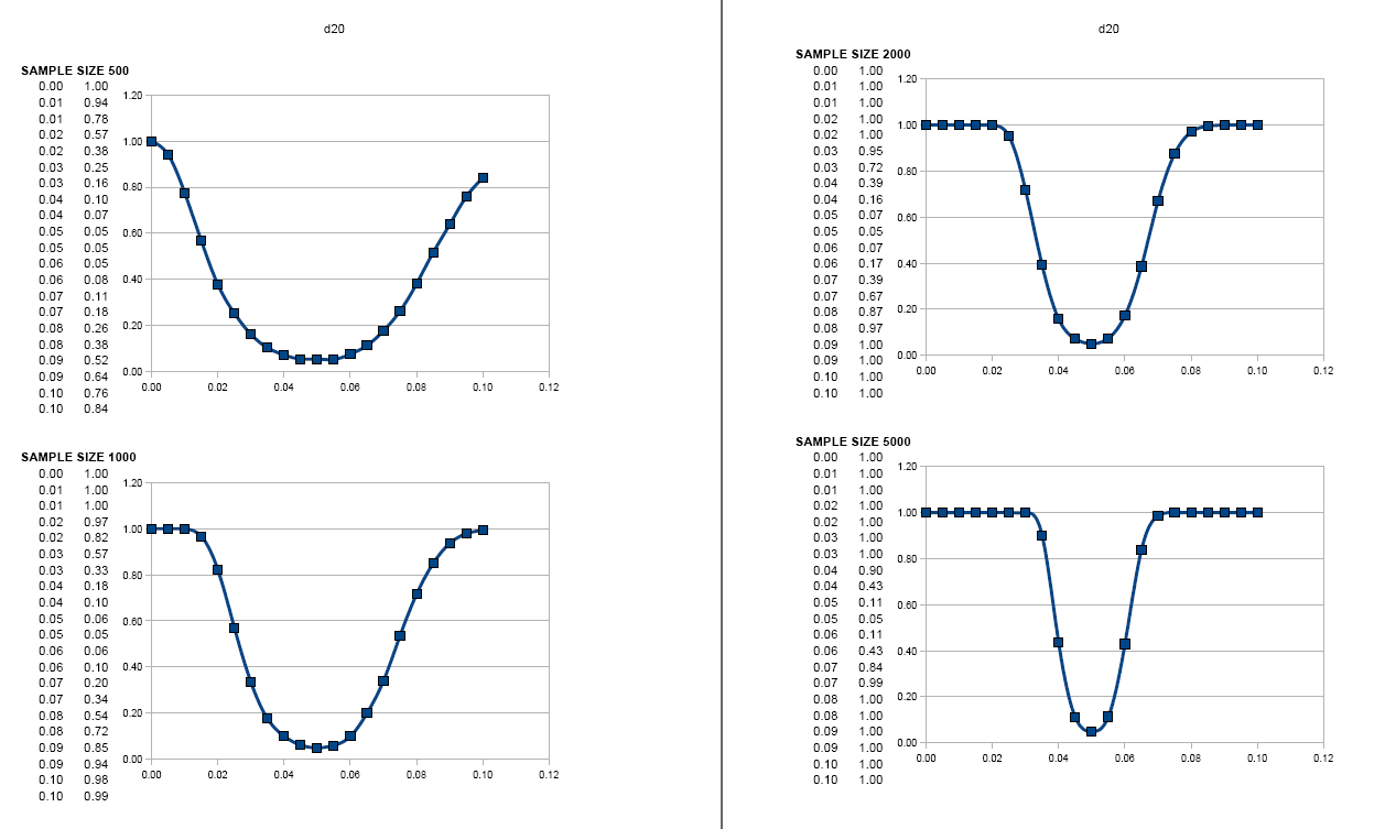 Here, I didn't even bother to show anything less than n=500, since the curves below that point are just dreadful (shown in the PDF again linked here). For example, at n=100 (previously the nominal minimum number of rolls), the chance of the test detecting the difference between a d19 and a d20 (i.e. one face missing) is only 16%! So in this case, although we have the same low false positive rate of α=5%, we have a sky-high false negative rate of β=84%. While a finding of "unbalanced" is one that we can count on, a finding of "not unbalanced" tells us almost nothing: it would usually do that anyway, even for a die entirely missing one or more faces.
This is honestly not something that I realized before doing the simulation experiment.
Take-away lesson is this, I think: The bare-minimum number of rolls given previously (5 times faces on the die) is pretty much useless for the test to be powerful enough to actually detect an unbalanced die. For a d6, I wouldn't want to use any less than n=100 as a minimum (and ideally something like n=500 if you're serious about it). For a d20, n=500 would be a useful minimum (and at least several thousand to find reasonably small variations). So realize that it takes a lot of rolling to have a chance of actually detecting unbalanced dice; look at the charts above and decide for yourself how small a bias you want to have a chance of identifying.
Postscript: Again, this is an analysis that is frequently overlooked, and if you got through this whole post, then you probably have a deeper understanding of the power of Pearson's chi-square test than even some professional statisticians (I dare say). For example, in the old Dragon magazine article on the subject (Dragon #78, Oct-1983), writer D.G. Weeks completely screwed up on this point. He wrote:
If your chi-square is less than the value in column one (labelled .10), the die is almost certainly fair (or close enough for any reasonable purpose).Well, that's just totally false. At minimal sample sizes, the test is of such low power, that the die can be almost certainly unfair and still pass the criteria. Furthermore, Weeks presented the possibility of a test for a given suspected die-face frequency and included it in the attached BASIC computer program, in doing so vastly confusing the issue of what's the null and what's the alternative hypothesis. To wit:
In this case it might make more sense to test directly whether this observation is really accurate, rather than simply making the general test described earlier. If what you suspect is true, a specialized test will show the bias more readily...What I would say is that this would actually prove the bias LESS readily, since your suspicion has now become the null hypothesis, and non-rejection of the null hypothesis tells us next to nothing about the die -- because that's what happens by default anyway, and the test is so very low-powered. In fact, Weeks is making precisely the mistake that we are being warned about by Professor Lowry in the quote at the very top of this blog post (read more at that link if you like: "it is a terrible idea to accept the null hypothesis upon failing to find a significant result in a one-dimensional chi-square test..."). Don't you make the same error!